Nov 5, 2015 • 7 min read
Draw smooth curves through a set of points

Sometime back, I came across this interesting challenge while working on an application. The app wanted to represent a particular set of data in a normal distribution graph.
Drawing regular line graphs are pretty straight forward. You just keep doing -addLineToPath(point:) to a Bézier path while iterating through the given points. For this problem I would need a curve instead of a line. I know the UIBezierPath class has these two methods :-
func addQuadCurveToPoint(endPoint: CGPoint, controlPoint: CGPoint)
func addCurveToPoint(endPoint: CGPoint, controlPoint1: CGPoint, controlPoint2: CGPoint)
So in this case we just use one of the functions for each point in the set? Do we use quadratic or cubic Bézier curve? How do we decide the control points? I had to do some magic to get it work.
Some Theory
While we can draw curves with ease freehand, computers are a bit handicapped in that they require some constraints to draw the curve we desire, since the number of curves that can be drawn from one point to an other is infinite. That’s where the control points come in to picture. They determine the curvature of the desired curve.
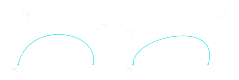
The curve from point P₀ to P₃ gets its shape from the control points P₁ and P₂.
If you’re interested in knowing how the curve is formed, check out this video and this animation.
Drawing poly-Bézier curves
A quadratic curve has one control point whereas a cubic curve has 2 control points to define its curvature. So basically, higher the degree, higher the number of control points required to defined the curve. Since higher degree curves are computationally expensive to evaluate, we restrict to mostly cubic and quadratic curves in computer graphics. When more complex shapes are needed, low order Bézier curves are chained together, to produce a poly-Bézier curve.
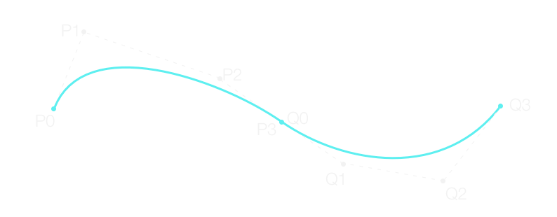
While compositing smooth Bézier curves, we need to ensure certain conditions -
- The end points of each section is the starting point of the next section (i.e. P₃ = Q0)
- The slope of the line connecting the last control point and the end point of a segment (P₂-P₃) should match the slope of the line connecting the starting point and first control point of the following segment (Q0-Q1). To simple put, the points P₂ — P₃/Q0 — Q1 should be collinear.
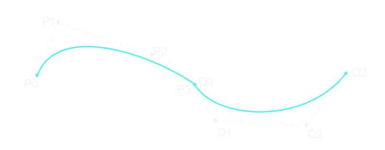
The second condition is important for a smooth composite curve, otherwise we would end up with a curve like so -
Cubic vs Quadratic
Using quadratic curves are ill-suited for a poly-Bézier curve, as all the control points are sort of linked. Altering one control point drastically affects other control points. So we’re going to use cubic curves as it allows more control over the curvature.
Back to the problem
Now that we have a basic understanding of Bézier curves, let’s tackle the problem. A cubic Bézier curve is given by,

where,
- P₀ and P₃ are the endpoints of a curve segment and P₁, P₂ are the control points.
- the parameter
t, is a fractional value which ranges from0to1. For a particular segment,B(0)refers to the starting point of the segment (P₀) andB(1)refers to the end point of the segment (P₃).
The equation can be rewritten as

Now if you recollect condition #2, the slopes at the dual point should match. Mathematically, slope is represented by the first derivative. So differentiating Eq. 01 gives,

For i-th segment, the slope at starting of the curve should be same as slope at the end of the (i-1)-th segment
Substituting the parameter t for 0 and 1 in Eq. 02,

Since the segments should be continuous and making use of condition #1 we discussed before,
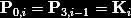
where K-i is the i-th point in the set. And using this back in Eq. 04,
A note on derivatives
The derivative of an n-th degree Bézier curve is an (n-1)-th degree Bézier curve. So the derivative of a cubic Bézier curve is a quadratic curve. The second derivative cubic curve will be,

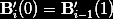
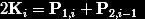
So the second derivative of the cubic curve should also be continuous. So at the segment ends we have,

Let’s use condition#1 and simply the equation to

The Eq.04 & Eq. 07, are defined for points where two segments come together. So we have 2(n-1) equations for 2n unknowns. Which means we need two more equations to get a proper solution.
Extremities
We can find the extremities of our poly-Bézier curve by solving equations B"(t) = 0 at the end points, i.e. B”(0) = 0 for the first segment & B”(1) = 0 for the last segment. Using these natural boundary conditions we get,


In Eq. 07, Eq. 08 and Eq. 09, replace the value of P₂ from Eq. 04 to get —


So these equations now involve only P₁ and the given set of points. We can solve using the Tridiagonal Matrix Algorithm without any tricks.
Similarly, we can setup equations for P₂,


Since we already have all the P₁ values, we can get P₂. That’s it! These are all the equations we need.
You wouldn’t clap yet, because proving something with equations is not good enough. You have to make it work. That’s why every magic trick has a third and final act.
Putting it together
It’s time to get our hands dirty. So we’ll solve for the first control points (P₁) for each segment and then the second control points.
First Control Points
var rhsArray = [CGPoint]()
var a = [Double]()
var b = [Double]()
var c = [Double]()
The rhsArray holds the RHS values from the Eq. 10a, 10b, 10c and the variables a, b, c hold the coefficients of the same.
for i in 0..<count {
    var rhsValueX: CGFloat = 0
    var rhsValueY: CGFloat = 0

    let P0 = dataPoints[i];
    let P3 = dataPoints[i+1];

    if i == 0 {
      a.append(0)
      b.append(2)
      c.append(1)

      //rhs for first segment
      rhsValueX = P0.x + 2*P3.x;
      rhsValueY = P0.y + 2*P3.y;
    } else if i == count-1 {
      a.append(2)
      b.append(7)
      c.append(0)

      //rhs for last segment
      rhsValueX = 8*P0.x + P3.x;
      rhsValueY = 8*P0.y + P3.y;
    } else {
      a.append(1)
      b.append(4)
      c.append(1)

      rhsValueX = 4*P0.x + 2*P3.x;
      rhsValueY = 4*P0.y + 2*P3.y;
    }

    rhsArray.append(CGPoint(x: rhsValueX, y: rhsValueY))
}
Now that we have the RHS values, we can solve for Ax = B, using the Tridiagonal matrix algorithm a.k.a Thomas Algorithm.
for i in 1..<count {
    let rhsValueX = rhsArray[i].x
    let rhsValueY = rhsArray[i].y

    let prevRhsValueX = rhsArray[i-1].x
    let prevRhsValueY = rhsArray[i-1].y

    let m = a[i]/b[i-1]

    let b1 = b[i] — m * c[i-1];
    b[i] = b1

    let r2x = rhsValueX — m * prevRhsValueX
    let r2y = rhsValueY — m * prevRhsValueY

    rhsArray[i] = CGPoint(x: r2x, y: r2y)
}
Get the first control points,
//Control Point of last segment
let lastControlPointX = rhsArray[count-1].x/b[count-1]
let lastControlPointY = rhsArray[count-1].y/b[count-1]

firstControlPoints[count-1] = CGPoint(x: lastControlPointX, y: lastControlPointY)

for i in (0...count-2).reversed() {
    if let nextControlPoint = firstControlPoints[i+1] {
      let controlPointX = (rhsArray[i].x — c[i] * nextControlPoint.x)/b[i]
      let controlPointY = (rhsArray[i].y — c[i] * nextControlPoint.y)/b[i]

      firstControlPoints[i] = CGPoint(x: controlPointX, y: controlPointY)
    }
}
Lastly, we compute the second control points from the first.
for i in 0..<count {
    if i == count-1 {
      let P3 = dataPoints[i+1]
      guard let P1 = firstControlPoints[i] else{
        continue
      }
      let controlPointX = (P3.x + P1.x)/2
      let controlPointY = (P3.y + P1.y)/2

      secondControlPoints.append(CGPoint(x: controlPointX, y: controlPointY))
    } else {
      let P3 = dataPoints[i+1]
      guard let nextP1 = firstControlPoints[i+1] else { continue }

      let controlPointX = 2*P3.x — nextP1.x
      let controlPointY = 2*P3.y — nextP1.y
      secondControlPoints.append(CGPoint(x: controlPointX, y: controlPointY))
    }
}
That’s the crux of the code. Compile and run, it should look like this..
Check out the source code here.
References
- @particleincell — For the crisp and clear equations.
- @pnowelldesign — For the video and animations.
- Primer on Bézier curves — For entire theory on Bézier curve.